How to use R with Cognite Data Fusion [Cognite Official]

R is a programming language and environment for statistical computing and graphics. It was developed in the 1990s by statisticians Ross Ihaka and Robert Gentleman and has since become one of the most widely used programming languages for data science. R is an open-source project, which means that anyone can contribute to its development and use it for free.

R is particularly popular among data scientists because of its powerful built-in tools for data manipulation, analysis, and visualization. R has a wide range of packages that can be used to perform various tasks in data science, such as data cleaning, statistical modelling, machine learning, and data visualization. R also has a highly active and supportive community, which means that there are many resources available online for learning and troubleshooting.

Fetching live data from Cognite Data Fusion in R can provide data scientists and analysts with a powerful tool for analysing and visualizing industrial data. It can help them identify trends, optimize processes, and improve overall efficiency, all while leveraging R’s extensive ecosystem of packages and tools.

Currently, there is no specific SDK for fetching data from Cognite Data Fusion in R. Therefore, in this guide, I will describe how to use the R library reticulate to utilize the Cognite Python SDK for fetching data.

Table of contents

What you should know

• Some experience using the terminal (command line) - you can read this tutorial on how to get started working with the command line for linux (most of it applies to the mac terminal as well).
• Some experience with R to understand the R syntax, and it's data structures - you can check the amazing R for Data Science online book to get started with R.
• Some experience working with Cognite Data Fusion data types and the Python SDK - you can read about resource types in the Cognite Documentation and how to use the Python SDK in the Cognite Python SDK Documentation.

Requirements

In this guide we'll be writing and running our R code from Jupyter notebooks. Optionally, you can install RStudio to write and run your R scripts.

Note: This guide has been tested in a mac, but it should work without problems in most linux environments. For Windows, I recommend using WSL to setup a linux environment. Let me know in the comments if you encountered any problems with the setup.

R

You must have R installed on your system. You can download the latest version of R from the R project website. Follow the instructions on the project website according to your platform.

Python

In order to use the R library reticulate and the Cognite Python SDK, you must have Python installed on your system.

Note:  reticulate requires a version of Python that has been compiled with shared library support (i.e. with the --enable-shared flag).

Miniconda is a bundle that has been tested and works great with reticulate.  You can download the latest version of miniconda from the project website. Follow the instructions on the project website according to your platform.

Python dependencies

After your miniconda runtime has been successfully installed, you can install the Python dependencies by running the following command from a terminal:

python -m pip install cognite-sdk pandas jupyterlab

Note: Make sure to run this command using the Python runtime from the miniconda distribution. By default, the miniconda installation makes the conda Python runtime the default Python in your system.

R dependencies

Next we'll be installing the R kernel for Jupyter and reticulate. Start by opening and R REPL by typing R and pressing enter in a terminal. Run the following commands in the R session:

install.packages("reticulate") 
install.packages('IRkernel')
IRkernel::installspec()

Getting started

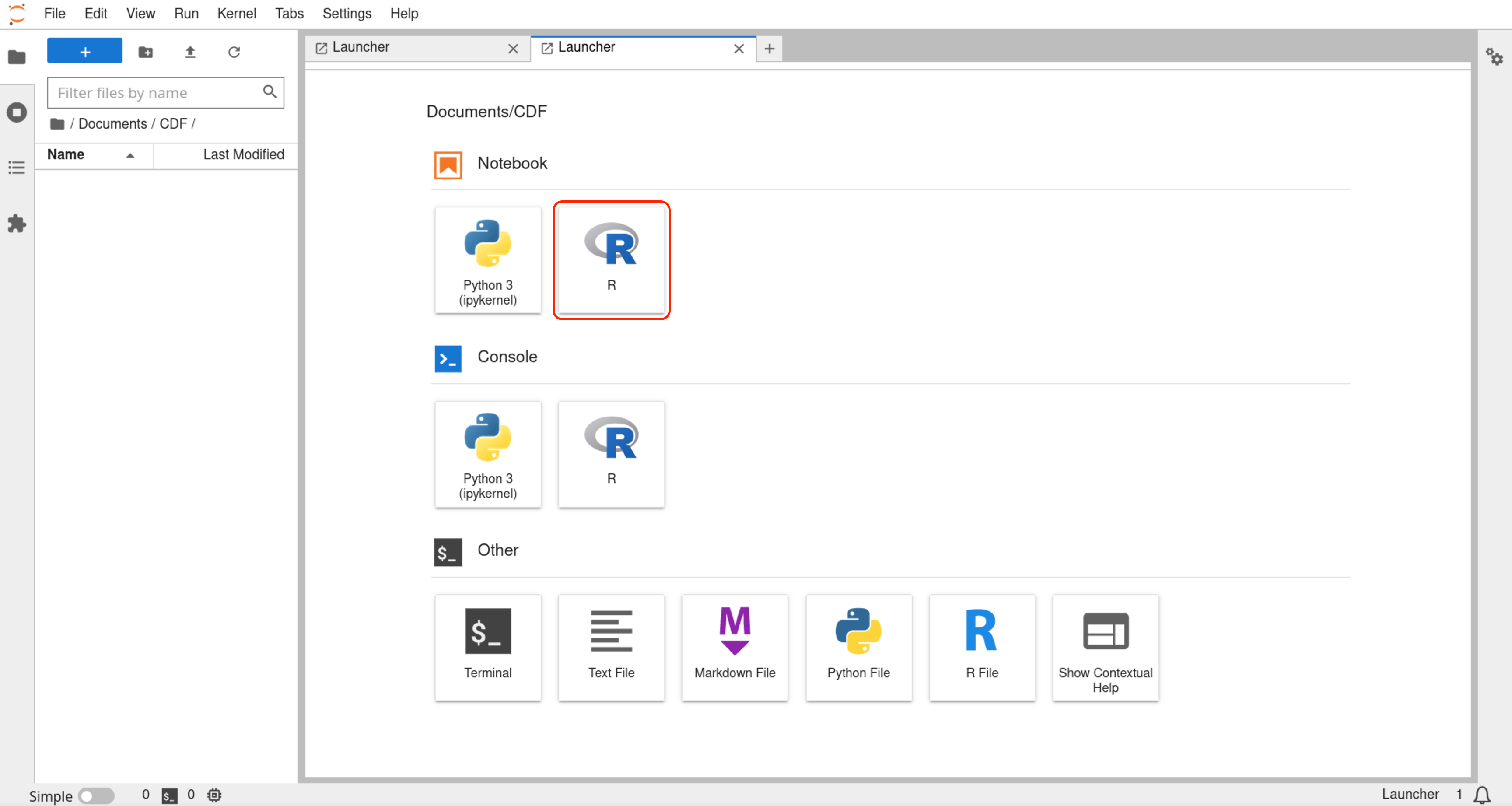
We'll be using a Jupyter notebook environment to write and run our R code. Navigate to a folder where you want to save your code and start Jupyter Lab by running jupyter lab in the terminal.

In Jupyter Lab create a new R notebook.

We'll start by storing the variables needed to authenticate to a Cognite Data Fusion (CDF) project. In this guide we'll be using an interactive flow, where a new browser tab will open and guide you through the process of authentication. 

client_id <- "client_id_goes_here"
tenant_id <- "tenant_id_goes_here"
cluster <- "cdf_cluster_goes_here"
project <- "cdf_project_goes_here"

If you don't know these variables, contact the administrator of the CDF project you want to connect to. If you don't have access to any CDF project, but just want to test this out, you can use the Open Industrial Data project called publicdata. Head to this link, create a free account to be able to authenticate to CDF in this project. After that, you can find the required variables to log into publicdata here.

Optional: If you want to share this notebook with colleagues, or make it public, it's recommended to store your authentication variables in an external file and importing it into the notebook, keeping them secret. A good practice is to store the variables in a .env file and using the R library dotenv to extract this variables as environment variables that can be accessed from the notebook.

Create a `.env` file and save the authentication variables as below

TENANT_ID=xxxx
CLIENT_ID=xxxx
CDF_CLUSTER=xxxx
CDF_PROJECT=xxxx

In an R session (or in an R notebook) run the command install.packages("dotenv")

In the R notebook run the following commands to read the variables from the .env file and store them into the associated R variables:

library(dotenv)
client_id <- as.character(Sys.getenv("CLIENT_ID"))
tenant_id <- as.character(Sys.getenv("TENANT_ID"))
cluster <- as.character(Sys.getenv("CDF_CLUSTER"))
project <- as.character(Sys.getenv("CDF_PROJECT"))

Now we will import reticulate, which will allow us to call Python from R. We also will define the path for the python runtime which contains the dependencies that we have already installed. Find the path for the python runtime in your system by running the command which python in a terminal and use it to replace the path in the command use_python below.

library(reticulate)
use_python(".../miniconda3/bin/Python")

With reticulate imported and the python runtime defined we can start working with the Cognite Python SDK. To simplify the process, I have created a simple function that handles the interactive authentication to CDF and instantiates a client. You can either define the function directly in the notebook or save it on an external R file and import it into the notebook by using the source function.

instantiate_cognite_client <- function(client_id, tenant_id, cluster, project) {
   scopes <- sprintf('https://%s.cognitedata.com/.default', cluster)
   base_url <- sprintf('https://%s.cognitedata.com', cluster)
   authority_url <- sprintf('https://login.microsoftonline.com/%s', tenant_id)

   py_run_string('from cognite.client import CogniteClient, ClientConfig')
   py_run_string('from cognite.client.credentials import OAuthInteractive')

   cred <- sprintf('creds = OAuthInteractive(authority_url="%s",client_id="%s",scopes=["%s"])', authority_url, client_id, scopes)
   py_run_string(cred)

   cnf <- sprintf('cnf = ClientConfig(client_name="test_notebook",project="%s",credentials=creds,base_url="%s")',project, base_url)
   py_run_string(cnf)

   py_run_string('client = CogniteClient(cnf)')

Note that this function will take the authentication variables from the R workspace and use them to instantiate a CDF client in the Python runtime being used by reticulate. We'll be using this client to fetch the data. After defining the function you can authenticate and instantiate the client by calling the function. A new browser tab should open, allowing you to log in into the IDP associated with the CDF project.

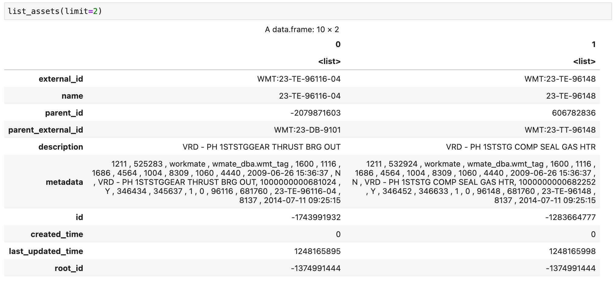
instantiate_cognite_client(client_id, tenant_id, cluster, project)

We can start testing our client by trying to retrieve some assets. Here as well, I'll be defining a simple function to handle the Python operations and returning an object that is compatible with R. This function can be extended to handle any parameters needed for your query.

list_assets <- function(limit) {
   request <- sprintf('assets_list = client.assets.list(limit=%s).to_pandas().T',limit)
   py_run_string(request)
   return(py$assets_list)
}

Notice that the return statement from the Python runtime is a Pandas DataFrame which is automatically converted to an R data.frame by the reticulate library. We can try the function by calling it to retrieve 2 assets.

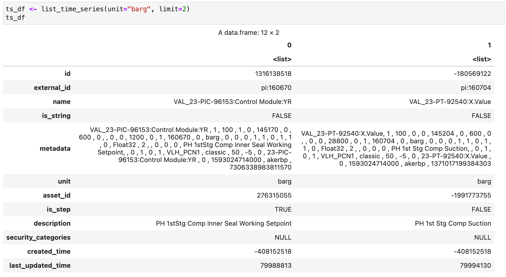
Now we can move on to time series. Below I'm defining two functions, one to list time series and another one to retrieve data points from a selected time series. Again, these functions are just an example and can be easily extended to handle different queries.

list_time_series <- function(unit, limit) {
   request <- sprintf('ts_list = client.time_series.list(unit="%s", limit=%s).to_pandas().T', unit, limit)
   py_run_string(request)
   return(py$ts_list)
}

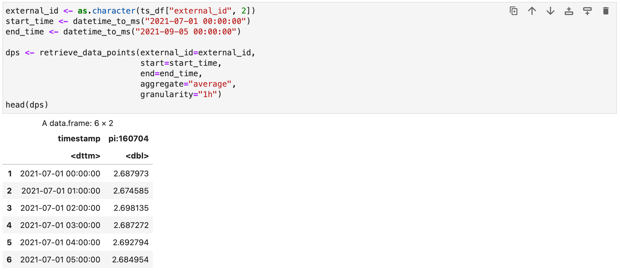
retrieve_data_points <- function(external_id, start, end, aggregate="average", granularity="1m") {
   request <- sprintf('dps = client.time_series.data.retrieve_dataframe( external_id="%s", start=%s, end=%s, aggregates=["%s"], granularity="%s", limit=None, include_aggregate_name=False)', external_id, start, end, aggregate, granularity)
   py_run_string(request)
   py_run_string('dps.reset_index(names="timestamp", inplace=True)')
   return(py$dps)
}

Now we can list the time series that have unit barg in the CDF project. For this example I'll limit the list to 2 instances:

Now we can download and plot some data points from a selected time series.

But first let's declare a function to simplify our work with timestamps. Timestamps in CDF are stored in UTC and are referenced using ms since epoch, which is not a practical reference for humans. The function below parses a timestamp in text format (assumed to be in UTC) to the associated ms since epoch.

datetime_to_ms <- function(timestamp, format="%Y-%m-%d %H:%M:%S") {
   dt <- as.POSIXct(timestamp, format = format)
   seconds_epoch <- as.numeric(dt)
   ms_epoch <- seconds_epoch * 1000 
   return(ms_epoch)
}

Now we can download some data points from the second time series that was retrieved in the previous CDF request.

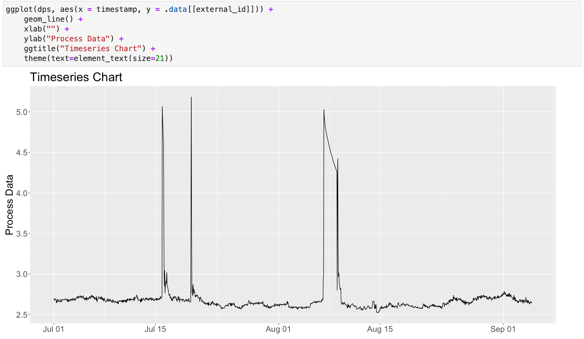
To visualize the data points we can use a plotting library like ggplot2. If it has not been installed yet in your R environment, you can do so by running install.packages("ggplot2") in an R session or directly in the notebook.

Once the library has been installed, we need to import it into our session. In the example below, I'm also defining the width and height of the plots for this session.

library(ggplot2)
library(repr)
options(repr.plot.width=16, repr.plot.height=8)

Now we can create a simple plot to visualize the data.

Final remarks

In this guide we have configured our R, Python and Jupyter environments, authenticated a CDF client, downloaded some data and visualized the data using an R library. This is just a simple example, to help get you started. From now on, you should be able to have a live connection to CDF and create amazing data insights and solutions using the powerful ecosystem of R. 

Let me know in the comments if you are facing some issues to follow the guide and if this type of content is interesting and relevant to you. If there is some interest, I can create a more elaborate example on how to create an R Shiny application with CDF data.